Compute lesion overlap
# ConWhAt stuff
from conwhat import VolConnAtlas,StreamConnAtlas,VolTractAtlas,StreamTractAtlas
from conwhat.viz.volume import plot_vol_scatter

# Neuroimaging stuff
import nibabel as nib
from nilearn.plotting import (plot_stat_map,plot_surf_roi,plot_roi,
                             plot_connectome,find_xyz_cut_coords)
from nilearn.image import resample_to_img

# Viz stuff
%matplotlib inline
from matplotlib import pyplot as plt
import seaborn as sns

# Generic stuff
import glob, numpy as np, pandas as pd, networkx as nx
from datetime import datetime
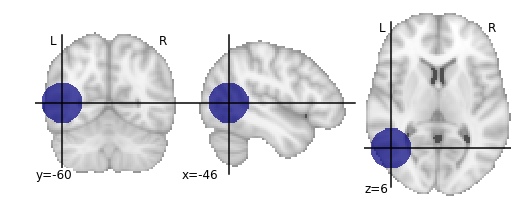
We now use the synthetic lesion constructed in the previous example in a ConWhAt lesion analysis.
lesion_file = 'synthetic_lesion_20mm_sphere_-46_-60_6.nii.gz' # we created this file from scratch in the previous example
Take another quick look at this mask:
lesion_img = nib.load(lesion_file)
plot_roi(lesion_file);
Since our lesion mask does not (by construction) have a huge amount of spatial detail, it makes sense to use one of the lower-resolution atlas. As one might expect, computation time is considerably faster for lower-resolution atlases.
>>> cw_atlases_dir = '/global/scratch/hpc3230/Data/conwhat_atlases'  # change this accordingly
>>> atlas_name = 'CWL2k8Sc33Vol3d100s_v01'
>>> atlas_dir = '%s/%s' %(cw_atlases_dir, atlas_name)
See the previous tutorial on ‘exploring the conwhat atlases’ for more info on how to examine the components of a given atlas in ConWhAt.
Initialize the atlas
>>> cw_vca = VolConnAtlas(atlas_dir=atlas_dir)
loading file mapping
loading vol bbox
loading connectivity
Choose which connections to evaluate.
This is normally an array of numbers indexing entries in
cw_vca.vfms.
Pre-defining connection subsets is a useful way of speeding up large analyses, especially if one is only interested in connections between specific sets of regions.
As we are using a relatively small atlas, and our lesion is not too extensive, we can assess all connections.
>>> idxs = 'all' # alternatively, something like: range(1,100), indicates the first 100 cnxns (rows in .vmfs)
Now, compute lesion overlap statistics.
>>> jlc_dir = '/global/scratch/hpc3230/joblib_cache_dir' # this is the cache dir where joblib writes temporary files
>>> lo_df,lo_nx = cw_vca.compute_hit_stats(lesion_file,idxs,n_jobs=4,joblib_cache_dir=jlc_dir)
computing hit stats for roi synthetic_lesion_20mm_sphere_-46_-60_6.nii.gz
This takes about 20 minutes to run.
vca.compute_hit_stats() returns a pandas dataframe, lo_df,
and a networkx object, lo_nx.
Both contain mostly the same information, which is sometimes more useful in one of these formats and sometimes in the other.
lo_df is a table, with rows corresponding to each connection, and
columns for each of a wide set of statistical
metrics
for evaluating sensitivity and specificity of binary hit/miss data:
>>> lo_df.head()
| metric | ACC | BM | F1 | FDR | FN | FNR | FP | FPR | Kappa | MCC | MK | NPV | PPV | TN | TNR | TP | TPR | corr_nothr | corr_thr | corr_thrbin |
|---|---|---|---|---|---|---|---|---|---|---|---|---|---|---|---|---|---|---|---|---|
| idx | ||||||||||||||||||||
| 0 | 0.990646 | 0.104859 | 0.098135 | 0.911501 | 29696.0 | 0.889874 | 37851.0 | 0.005266 | 0.330534 | 0.094054 | 0.084363 | 0.995864 | 0.088499 | 7149810.0 | 0.994734 | 3675.0 | 0.110126 | 0.042205 | 0.042205 | 0.094054 |
| 3 | 0.987324 | 0.011683 | 0.014279 | 0.988855 | 32708.0 | 0.980132 | 58828.0 | 0.008185 | 0.329134 | 0.008766 | 0.006577 | 0.995433 | 0.011145 | 7128833.0 | 0.991815 | 663.0 | 0.019868 | -0.001487 | -0.001487 | 0.008766 |
| 7 | 0.987160 | -0.006617 | 0.001185 | 0.999075 | 33316.0 | 0.998352 | 59404.0 | 0.008265 | 0.329023 | -0.004966 | -0.003727 | 0.995348 | 0.000925 | 7128257.0 | 0.991735 | 55.0 | 0.001648 | -0.003549 | -0.003549 | -0.004966 |
| 10 | 0.994367 | -0.000926 | 0.000147 | 0.999589 | 33368.0 | 0.999910 | 7305.0 | 0.001016 | 0.331450 | -0.001976 | -0.004215 | 0.995374 | 0.000411 | 7180356.0 | 0.998984 | 3.0 | 0.000090 | -0.001975 | -0.001975 | -0.001976 |
| 11 | 0.989105 | 0.048907 | 0.044941 | 0.962227 | 31520.0 | 0.944533 | 47152.0 | 0.006560 | 0.329846 | 0.040403 | 0.033378 | 0.995605 | 0.037773 | 7140509.0 | 0.993440 | 1851.0 | 0.055467 | 0.017664 | 0.017664 | 0.040403 |
Typically we will be mainly interested in two of these metric scores:
TPR - True positive (i.e. hit) rate: number of true positives,
divided by number of true positives + number of false negatives
corr_thrbin - Pearson correlation between the lesion amge and the
thresholded, binarized connectome edge image (group-level visitation
map)
>>> lo_df[['TPR', 'corr_thrbin']].iloc[:10].T
| idx | 0 | 3 | 7 | 10 | 11 | 13 | 14 | 15 | 18 | 19 |
|---|---|---|---|---|---|---|---|---|---|---|
| metric | ||||||||||
| TPR | 0.110126 | 0.019868 | 0.001648 | 0.000090 | 0.055467 | 0.002128 | 0.000569 | 0.000000 | 0.098469 | 0.023523 |
| corr_thrbin | 0.094054 | 0.008766 | -0.004966 | -0.001976 | 0.040403 | 0.005801 | 0.000641 | -0.002543 | 0.169234 | 0.029414 |
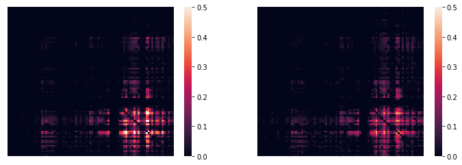
We can obtain these numbers as a ‘modification matrix’ (connectivity matrix)
>>> tpr_adj = nx.to_pandas_adjacency(lo_nx,weight='TPR')
>>> cpr_adj = nx.to_pandas_adjacency(lo_nx,weight='corr_thrbin')
These two maps are, unsurprisingly, very similar:
>>> np.corrcoef(tpr_adj.values.ravel(), cpr_adj.values.ravel())
array([[1.        , 0.96271946],
       [0.96271946, 1.        ]])
>>> fig, ax = plt.subplots(ncols=2, figsize=(12,4))
>>> sns.heatmap(tpr_adj,xticklabels='',yticklabels='',vmin=0,vmax=0.5,ax=ax[0]);
>>> sns.heatmap(cpr_adj,xticklabels='',yticklabels='',vmin=0,vmax=0.5,ax=ax[1]);
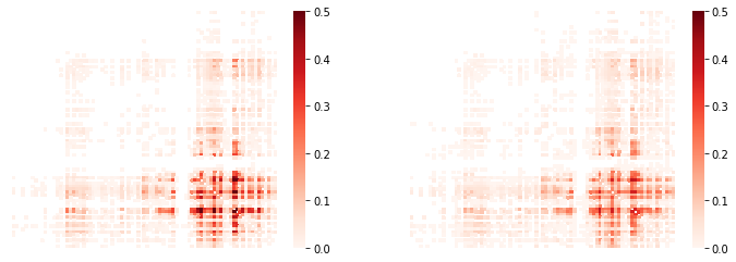
(…with an alternative color scheme…)
>>> fig, ax = plt.subplots(ncols=2, figsize=(12,4))
>>> sns.heatmap(tpr_adj, xticklabels='',yticklabels='',cmap='Reds',
>>>                   mask=tpr_adj.values==0,vmin=0,vmax=0.5,ax=ax[0]);
>>> sns.heatmap(cpr_adj,xticklabels='',yticklabels='',cmap='Reds',
>>>                   mask=cpr_adj.values==0,vmin=0,vmax=0.5,ax=ax[1]);
We can list directly the most affected (greatest % overlap) connections,
>>> cw_vca.vfms.loc[lo_df.index].head()
| name | nii_file | nii_file_id | 4dvolind | |
|---|---|---|---|---|
| idx | ||||
| 0 | 61_to_80 | vismap_grp_62-81_norm.nii.gz | 0 | NaN |
| 3 | 18_to_19 | vismap_grp_19-20_norm.nii.gz | 3 | NaN |
| 7 | 45_to_48 | vismap_grp_46-49_norm.nii.gz | 7 | NaN |
| 10 | 19_to_68 | vismap_grp_20-69_norm.nii.gz | 10 | NaN |
| 11 | 21_to_61 | vismap_grp_22-62_norm.nii.gz | 11 | NaN |
To plot the modification matrix information on a brain, we first need to some spatial locations to plot as nodes. For these, we calculate (an approprixation to) each atlas region’s centriod location:
>>> parc_img = cw_vca.region_nii
>>> parc_dat = parc_img.get_data()
>>> parc_vals = np.unique(parc_dat)[1:]

>>> ccs = {roival: find_xyz_cut_coords(nib.Nifti1Image((dat==roival).astype(int),img.affine),
>>>                                   activation_threshold=0) for roival in roivals}
>>> ccs_arr = np.array(ccs.values())
Now plotting on a glass brain:
>>> fig, ax = plt.subplots(figsize=(16,6))
>>> plot_connectome(tpr_adj.values,ccs_arr,axes=ax,edge_threshold=0.2,colorbar=True,
>>>                    edge_cmap='Reds',edge_vmin=0,edge_vmax=1.,
>>>                    node_color='lightgrey',node_kwargs={'alpha': 0.4});
>>> #edge_vmin=0,edge_vmax=1)
>>> fig, ax = plt.subplots(figsize=(16,6))
>>> plot_connectome(cpr_adj.values,ccs_arr,axes=ax)
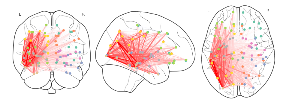
The lines in this figure show network connections (drawn as a straight line between two nodes) whose atlas image volume have a non-zero level of overlap with the synthetic lesion volume. Transparency and colour intensity indicate the magnitude of overlap. Thus the thickest, brightest red lines correspond to tracts that pass directly through the centre of the synthetic lesion mask, and for whom the lesion overlaps with a substantial amount of their total volume. Light, thinner lines, extending to/from the contralateral hemisphere and frontal cortex, correspond to connections with a proportionally smaller degree of lesion load.