Exploring ConWhAt Atlases
There are four different atlas types in ConWhat, corresponding to the 2 ontology types (Tract-based / Connectivity-Based) and 2 representation types (Volumetric / Streamlinetric).
(More on this schema here)
In [1]:
# ConWhAt stuff
from conwhat import VolConnAtlas,StreamConnAtlas,VolTractAtlas,StreamTractAtlas
from conwhat.viz.volume import plot_vol_scatter,plot_vol_and_rois_nilearn

# Neuroimaging stuff
import nibabel as nib
from nilearn.plotting import plot_stat_map,plot_surf_roi

# Viz stuff
%matplotlib inline
from matplotlib import pyplot as plt
import seaborn as sns

# Generic stuff
import glob, numpy as np, pandas as pd, networkx as nx
We’ll start with the scale 33 lausanne 2008 volumetric connectivity-based atlas.
Define the atlas name and top-level directory location
In [2]:
atlas_dir = '/scratch/hpc3230/Data/conwhat_atlases'
atlas_name = 'CWL2k8Sc33Vol3d100s_v01'
Initialize the atlas class
In [3]:
vca = VolConnAtlas(atlas_dir=atlas_dir + '/' + atlas_name,
                   atlas_name=atlas_name)
loading file mapping
loading vol bbox
loading connectivity
This atlas object contains various pieces of general information
In [9]:
vca.atlas_name
Out[9]:
'CWL2k8Sc33Vol3d100s_v01'
In [8]:
vca.atlas_dir
Out[8]:
'/scratch/hpc3230/Data/conwhat_atlases/CWL2k8Sc33Vol3d100s_v01'
Information about each atlas entry is contained in the vfms
attribute, which returns a pandas dataframe
In [14]:
vca.vfms.head()
Out[14]:
| name | nii_file | nii_file_id | 4dvolind | |
|---|---|---|---|---|
| 0 | 61_to_80 | vismap_grp_62-81_norm.nii.gz | 0 | NaN |
| 1 | 38_to_55 | vismap_grp_39-56_norm.nii.gz | 1 | NaN |
| 2 | 28_to_38 | vismap_grp_29-39_norm.nii.gz | 2 | NaN |
| 3 | 18_to_19 | vismap_grp_19-20_norm.nii.gz | 3 | NaN |
| 4 | 26_to_55 | vismap_grp_27-56_norm.nii.gz | 4 | NaN |
Additionally, connectivity-based atlases also contain a networkx
graph object vca.Gnx, which contains information about each
connectome edge
In [62]:
vca.Gnx.edges[(10,35)]
Out[62]:
{'attr_dict': {'4dvolind': nan,
  'fullname': 'L_paracentral_to_L_caudate',
  'idx': 1637,
  'name': '10_to_35',
  'nii_file': 'vismap_grp_11-36_norm.nii.gz',
  'nii_file_id': 1637,
  'weight': 50.240000000000002,
  'xmax': 92,
  'xmin': 61,
  'ymax': 167,
  'ymin': 75,
  'zmax': 92,
  'zmin': 62}}
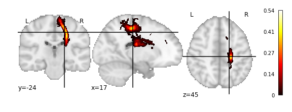
Individual atlas entry nifti images can be grabbed like so
In [144]:
img = vca.get_vol_from_vfm(1637)
getting atlas entry 1637: image file /scratch/hpc3230/Data/conwhat_atlases/CWL2k8Sc33Vol3d100s_v01/vismap_grp_11-36_norm.nii.gz
In [146]:
plot_stat_map(img)
Out[146]:
<nilearn.plotting.displays.OrthoSlicer at 0x7fb19fada410>
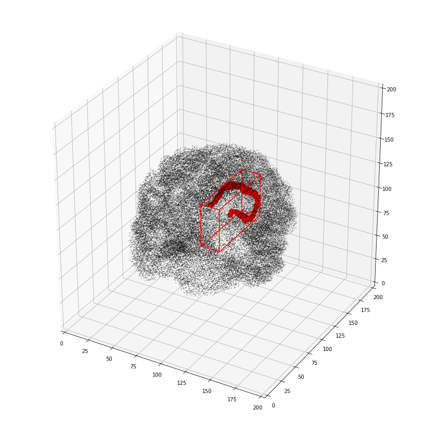
Or alternatively as a 3D scatter plot, along with the x,y,z bounding box
In [155]:
vca.bbox.ix[1637]
Out[155]:
xmin     61
xmax     92
ymin     75
ymax    167
zmin     62
zmax     92
Name: 1637, dtype: int64
In [134]:
ax = plot_vol_scatter(vca.get_vol_from_vfm(1),c='r',bg_img='nilearn_destrieux',
                      bg_params={'s': 0.1, 'c':'k'},figsize=(20, 15))

ax.set_xlim([0,200]); ax.set_ylim([0,200]); ax.set_zlim([0,200]);
getting atlas entry 1: image file /scratch/hpc3230/Data/conwhat_atlases/CWL2k8Sc33Vol3d100s_v01/vismap_grp_39-56_norm.nii.gz
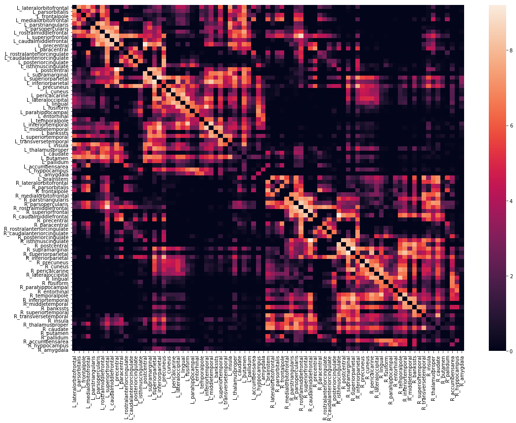
We can also view the weights matrix like so:
In [38]:
fig, ax = plt.subplots(figsize=(16,12))

sns.heatmap(np.log1p(vca.weights),xticklabels=vca.region_labels,
            yticklabels=vca.region_labels,ax=ax);
plt.tight_layout()
The vca object also contains x,y,z bounding boxes for each structure
We also stored additional useful information about the ROIs in the associated parcellation, including cortical/subcortical labels
In [156]:
vca.cortex
Out[156]:
array([ 1.,  1.,  1.,  1.,  1.,  1.,  1.,  1.,  1.,  1.,  1.,  1.,  1.,
        1.,  1.,  1.,  1.,  1.,  1.,  1.,  1.,  1.,  1.,  1.,  1.,  1.,
        1.,  1.,  1.,  1.,  1.,  1.,  1.,  1.,  0.,  0.,  0.,  0.,  0.,
        0.,  0.,  0.,  1.,  1.,  1.,  1.,  1.,  1.,  1.,  1.,  1.,  1.,
        1.,  1.,  1.,  1.,  1.,  1.,  1.,  1.,  1.,  1.,  1.,  1.,  1.,
        1.,  1.,  1.,  1.,  1.,  1.,  1.,  1.,  1.,  1.,  1.,  0.,  0.,
        0.,  0.,  0.,  0.,  0.])
…hemisphere labels
In [157]:
vca.hemispheres
Out[157]:
array([ 1.,  1.,  1.,  1.,  1.,  1.,  1.,  1.,  1.,  1.,  1.,  1.,  1.,
        1.,  1.,  1.,  1.,  1.,  1.,  1.,  1.,  1.,  1.,  1.,  1.,  1.,
        1.,  1.,  1.,  1.,  1.,  1.,  1.,  1.,  1.,  1.,  1.,  1.,  1.,
        1.,  1.,  1.,  0.,  0.,  0.,  0.,  0.,  0.,  0.,  0.,  0.,  0.,
        0.,  0.,  0.,  0.,  0.,  0.,  0.,  0.,  0.,  0.,  0.,  0.,  0.,
        0.,  0.,  0.,  0.,  0.,  0.,  0.,  0.,  0.,  0.,  0.,  0.,  0.,
        0.,  0.,  0.,  0.,  0.])
…and region mappings to freesurfer’s fsaverage brain
In [158]:
vca.region_mapping_fsav_lh
Out[158]:
array([ 24., 29., 28., ..., 16., 7., 7.])
In [159]:
vca.region_mapping_fsav_rh
Out[159]:
array([ 24., 29., 22., ..., 9., 9., 9.])
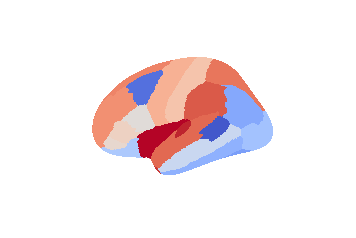
which can be used for, e.g. plotting ROI data on a surface
In [167]:
f = '/opt/freesurfer/freesurfer/subjects/fsaverage/surf/lh.inflated'
vtx,tri = nib.freesurfer.read_geometry(f)
plot_surf_roi([vtx,tri],vca.region_mapping_fsav_lh);